How Do I Find Missing Values In Two Columns In Excel

19 Nov, 2021

Then the matched values will give us the confirmation using the IF function. IFCOUNTIF list F6 OKMissing where list is the named range B6B11.

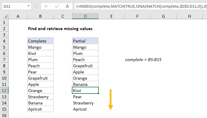
Excel Formula Find And Retrieve Missing Values Exceljet

If you want to compare and extract the missing values from two columns here is another formula to help you.

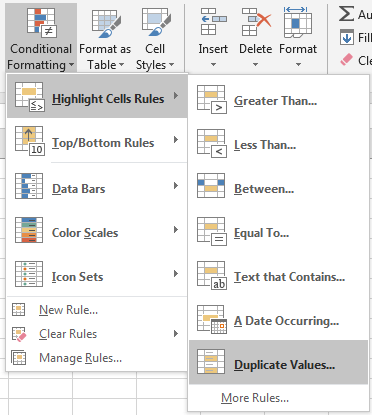
How do i find missing values in two columns in excel. Column C returns values from column A which are not present in column B. In the Styles group click on the Conditional Formatting option. Keep default value in values with.

It is a normal non-array formula which is to be entered. Type the number of columns your field is from the Unique ID where the Unique ID is 1. Select the entire data set.

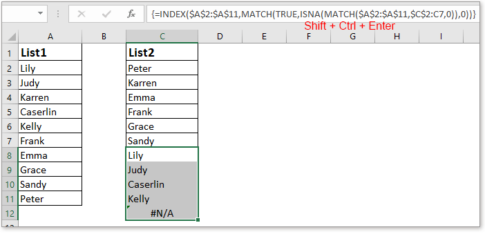
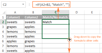
Select cell C2 by clicking on it. Compare and extract the missing values from two columns with formula. Summary To compare two lists and pull missing values from one list to the other you can use an array formula based on INDEX and MATCH.

Functions Used in this Formula make list of missing. You are correct - COLUMN C shows the values which are missing in column B but are in column A. Using the formula in F3 to look for the missing value in E3 in the list B3B8 The results of this formula can be observed in the snapshot below.

To find the missing value in the cell E3 enter the following formula in F3 to check its status. In the example shown the last value in list B is in cell D11. Filter A2A13isna match A2A13B2B110 into cell C2 and then press Enter key all values in List 1 but not in List 2 are extracted as following screenshot shown.

Compare Two Columns to Find Missing Value by Conditional Formatting. When you hide the column the only what Excel does is set the width of such column to zero. We need to match whether List A contains all the List.

In Duplicate Values dialog select Unique in dropdown list. Click the Home tab. IF COUNTIF listE3OKMISSING Figure2.

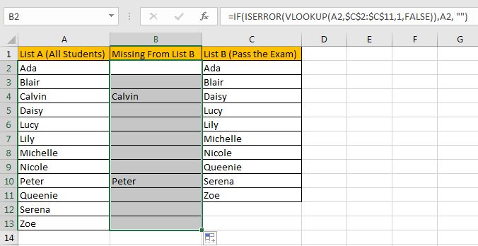
Insert the formula in IF ISERROR VLOOKUP A2B2B10011FALSEFALSETRUE the formula bar. List Missing Numbers in a Sequence With An Excel Formula. Click Home in ribbon click Conditional Formatting in Styles group.

You may download the excel file from below link wherein this has been illustrated. The cell reference in the ROW A1 part of the formula is relative so as you copy the formula down column C ROW A1 becomes ROW A2 which 2 and returns the second smallest missing number ROW A3 which is 3 returns the third smallest missing number and so on. Select the first blank cell besides Fruit List 2 type Missing in Fruit List 1 as column header next enter the formula IF ISERROR VLOOKUP A2Fruit List 1A2A221FALSEA2 into the second blank cell and drag the Fill Handle to the range as you need.

The formula in D12 copied down is. Rich99 its the same. The formula should not give a circular reference unless ranges overlap.

Two vertical lines shall indicate such column was it hide or manually set to zero width. Updated status of missing and available values. This identifies which column contains the information you want from Spreadsheet 2.

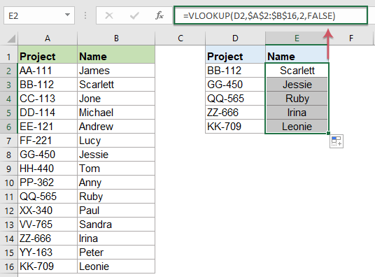
When the two columns data is lined up like the below we will use VLOOKUP to see whether column 1 includes column 2 or not. Unhide shall work in both cases. Firstly the lookup value is searched in the particular column of the table array.

Use of COUNTIF and IF function. Hover the cursor on the Highlight Cell Rules option. Go to Col_index_num click in it once.

The video offers a short tutorial on how to find missing values between two lists in Excel. Here the Email field is the third column. In the Format values where this formula is true field enter the formula.

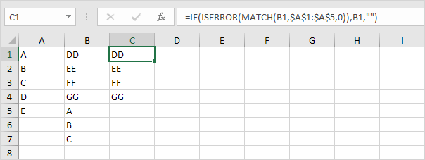
Otherwise it will leave the cell empty. If it doesnt find anything COUNFIF is equal to 0 means the B1 is in B but missing in A. In the example shown the formula in G6 is.

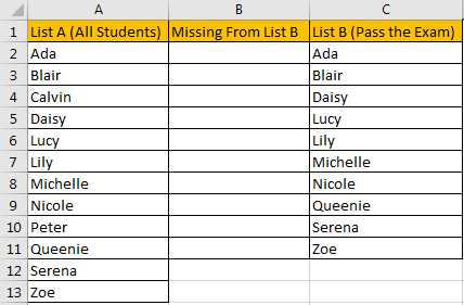
It will write the B1 value in the C1 cell. Press Enter to assign the formula to C2. Select List A and List B.

You can check if the values in column A exist in column B using VLOOKUP. The IF function returns the confirmation using the values Is there Missing. A2B2 Click on the Format button Click on the Fill tab and select the color in which you want to highlight the rows with the same value in both columns.

To identify values in one list that are missing in another list you can use a simple formula based on the COUNTIF function with the IF function. This formula searches through the A column for the B1 value. In Conditional Formatting dropdown list select Highlight Cells Rules-Duplicate Values.

Excel Formula Find Missing Values Exceljet

How To Compare Two Columns To Find Missing Value Unique Value In Excel Free Excel Tutorial

Group Data In An Excel Pivottable Pivot Table Excel Data

Display Missing Dates In Excel Pivottables My Online Training Hub Excel Dating Print Layout

How To Use Division Formula In Excel Microsoft Excel Excel Tutorials Microsoft Excel Tutorial

Compare Two Columns And Add Missing Values In Excel

How To Split A Cell In Excel How To Split Splits Cell

Compare Two Columns And Remove Duplicates In Excel Excel Excel Formula Microsoft Excel

How To Find Missing Items In A Column With Consecutive Numbers In Excel Worksheet Excel Excel Formula Column

How To Compare Two Columns To Find Missing Value Unique Value In Excel Free Excel Tutorial

Excel Compare Two Columns For Matches And Differences

How To Compare Two Columns And Return Values From The Third Column In Excel

How To Compare Two Columns For Highlighting Missing Values In Excel

Compare Two Columns Easy Excel Tutorial

Excel Pivot Tables Custom Calculations Pivot Table Free Workbook Excel Spreadsheets

How To Compare 2 Columns With Excel So Easy With Only 2 Functions

How To Compare Two Columns For Highlighting Missing Values In Excel